Cooley-Tukey FFT

In a previous article i briefly touched on FFTs. I mentioned that they are a faster way to perform polynomial interpolation. But FFTs are used for more than just polynomials. Specifically they are used for computing DFTs. A DFT is a system of linear equations that are related whose basis lies in $\mathbb{C}^n$. DFTs have other applications in signal processing.

In order to motivate the need for the FFT, Let’s examine a 12-degree polynomial in whose basis lies in the real.

$$\begin{aligned} P(x_0) &= a_0 + a_1x_0 + a_2x_0^2 + a_3x_0^3 + a_4x_0^4 + a_5x_0^5 + a_6x_0^6 + a_7x_0^7 + a_8x_0^8 + a_9x_0^9 + a_{10}x_0^{10} + a_{11}x_0^{11} \\ P(x_1) &= a_0 + a_1x_1 + a_2x_1^2 + a_3x_1^3 + a_4x_1^4 + a_5x_1^5 + a_6x_1^6 + a_7x_1^7 + a_8x_1^8 + a_9x_1^9 + a_{10}x_1^{10} + a_{11}x_1^{11} \\ P(x_2) &= a_0 + a_1x_2 + a_2x_2^2 + a_3x_2^3 + a_4x_2^4 + a_5x_2^5 + a_6x_2^6 + a_7x_2^7 + a_8x_2^8 + a_9x_2^9 + a_{10}x_2^{10} + a_{11}x_2^{11} \\ P(x_3) &= a_0 + a_1x_3 + a_2x_3^2 + a_3x_3^3 + a_4x_3^4 + a_5x_3^5 + a_6x_3^6 + a_7x_3^7 + a_8x_3^8 + a_9x_3^9 + a_{10}x_3^{10} + a_{11}x_3^{11} \\ P(x_4) &= a_0 + a_1x_4 + a_2x_4^2 + a_3x_4^3 + a_4x_4^4 + a_5x_4^5 + a_6x_4^6 + a_7x_4^7 + a_8x_4^8 + a_9x_4^9 + a_{10}x_4^{10} + a_{11}x_4^{11} \\ P(x_5) &= a_0 + a_1x_5 + a_2x_5^2 + a_3x_5^3 + a_4x_5^4 + a_5x_5^5 + a_6x_5^6 + a_7x_5^7 + a_8x_5^8 + a_9x_5^9 + a_{10}x_5^{10} + a_{11}x_5^{11} \\ P(x_6) &= a_0 + a_1x_6 + a_2x_6^2 + a_3x_6^3 + a_4x_6^4 + a_5x_6^5 + a_6x_6^6 + a_7x_6^7 + a_8x_6^8 + a_9x_6^9 + a_{10}x_6^{10} + a_{11}x_6^{11} \\ P(x_7) &= a_0 + a_1x_7 + a_2x_7^2 + a_3x_7^3 + a_4x_7^4 + a_5x_7^5 + a_6x_7^6 + a_7x_7^7 + a_8x_7^8 + a_9x_7^9 + a_{10}x_7^{10} + a_{11}x_7^{11} \\ P(x_8) &= a_0 + a_1x_8 + a_2x_8^2 + a_3x_8^3 + a_4x_8^4 + a_5x_8^5 + a_6x_8^6 + a_7x_8^7 + a_8x_8^8 + a_9x_8^9 + a_{10}x_8^{10} + a_{11}x_8^{11} \\ P(x_9) &= a_0 + a_1x_9 + a_2x_9^2 + a_3x_9^3 + a_4x_9^4 + a_5x_9^5 + a_6x_9^6 + a_7x_9^7 + a_8x_9^8 + a_9x_9^9 + a_{10}x_9^{10} + a_{11}x_9^{11} \\ P(x_{10}) &= a_0 + a_1x_{10} + a_2x_{10}^2 + a_3x_{10}^3 + a_4x_{10}^4 + a_5x_{10}^5 + a_6x_{10}^6 + a_7x_{10}^7 + a_8x_{10}^8 + a_9x_{10}^9 + a_{10}x_{10}^{10} + a_{11}x_{10}^{11} \\ P(x_{11}) &= a_0 + a_1x_{11} + a_2x_{11}^2 + a_3x_{11}^3 + a_4x_{11}^4 + a_5x_{11}^5 + a_6x_{11}^6 + a_7x_{11}^7 + a_8x_{11}^8 + a_9x_{11}^9 + a_{10}x_{11}^{10} + a_{11}x_{11}^{11} \\ \end{aligned}$$

It’s clear from writing out this expression that the complexity of calculating each $P(x_i)$ for $x \in \{0, \dots, n-1 \}$ is $O(N^2)$. Another way to look at this system of equations is through the lens of matrix multiplication:

$$\begin{bmatrix} 1 & x_0 & x_0^2 & x_0^3 & x_0^4 & x_0^5 & x_0^6 & x_0^7 & x_0^8 & x_0^9 & x_0^{10} & x_0^{11} \\ 1 & x_1 & x_1^2 & x_1^3 & x_1^4 & x_1^5 & x_1^6 & x_1^7 & x_1^8 & x_1^9 & x_1^{10} & x_1^{11} \\ 1 & x_2 & x_2^2 & x_2^3 & x_2^4 & x_2^5 & x_2^6 & x_2^7 & x_2^8 & x_2^9 & x_2^{10} & x_2^{11} \\ 1 & x_3 & x_3^2 & x_3^3 & x_3^4 & x_3^5 & x_3^6 & x_3^7 & x_3^8 & x_3^9 & x_3^{10} & x_3^{11} \\ 1 & x_4 & x_4^2 & x_4^3 & x_4^4 & x_4^5 & x_4^6 & x_4^7 & x_4^8 & x_4^9 & x_4^{10} & x_4^{11} \\ 1 & x_5 & x_5^2 & x_5^3 & x_5^4 & x_5^5 & x_5^6 & x_5^7 & x_5^8 & x_5^9 & x_5^{10} & x_5^{11} \\ 1 & x_6 & x_6^2 & x_6^3 & x_6^4 & x_6^5 & x_6^6 & x_6^7 & x_6^8 & x_6^9 & x_6^{10} & x_6^{11} \\ 1 & x_7 & x_7^2 & x_7^3 & x_7^4 & x_7^5 & x_7^6 & x_7^7 & x_7^8 & x_7^9 & x_7^{10} & x_7^{11} \\ 1 & x_8 & x_8^2 & x_8^3 & x_8^4 & x_8^5 & x_8^6 & x_8^7 & x_8^8 & x_8^9 & x_8^{10} & x_8^{11} \\ 1 & x_9 & x_9^2 & x_9^3 & x_9^4 & x_9^5 & x_9^6 & x_9^7 & x_9^8 & x_9^9 & x_9^{10} & x_9^{11} \\ 1 & x_{10} & x_{10}^2 & x_{10}^3 & x_{10}^4 & x_{10}^5 & x_{10}^6 & x_{10}^7 & x_{10}^8 & x_{10}^9 & x_{10}^{10} & x_{10}^{11} \\ 1 & x_{11} & x_{11}^2 & x_{11}^3 & x_{11}^4 & x_{11}^5 & x_{11}^6 & x_{11}^7 & x_{11}^8 & x_{11}^9 & x_{11}^{10} & x_{11}^{11} \\ \end{bmatrix} \begin{bmatrix} a_0 \\ a_1 \\ a_2 \\ a_3 \\ a_4 \\ a_5 \\ a_6 \\ a_7 \\ a_8 \\ a_9 \\ a_{10} \\ a_{11} \\ \end{bmatrix} = \begin{bmatrix} P(x_0) \\ P(x_1) \\ P(x_2) \\ P(x_3) \\ P(x_4) \\ P(x_5) \\ P(x_6) \\ P(x_7) \\ P(x_8) \\ P(x_9) \\ P(x_{10}) \\ P(x_{11}) \\ \end{bmatrix}$$

This matrix is also known as the vandermonde matrix. The vandermonde matrix is invertible, since it is a square matrix with distinct elements. This equation can therefore be re-arranged allowing us to derive the coefficients $a_i$s of the polynomial given the evaluations $P(x_i)$.

$$a = V^{-1}P$$

This is an alternative algebraic form of polynomial interpolation, other forms include Lagrange polynomials, Newton’s polynomials etc. Unfortunately, performing either operations, whether polynomial evaluation or interpolation leads to a complexity of $O(N^2)$.

Discrete Fourier Transform

The Fast Fourier Transform provides a way to transform the complexity of computing a DFT of size $N$ for which the naive approach takes $O(N^2)$ complexity into something quasilinear. In order for this to happen, we need to perform a change of basis, i.e rewrite the coordinates of our polynomial to be elements of a cyclic group. Such that they are indexed by successive powers of the generator of this cyclic group. Thus we get the DFT

$$\begin{equation} X(j) = \sum_{k = 0}^{N-1} A(k)\cdot \omega^{jk}, \quad j = 0,1,\dots N-1. \tag{1} \end{equation}$$

where $\omega = e^{2\pi i/N}$, such that $\omega^N = 1$. Let’s look at this in matrix form for $N = 12$.

$$\begin{bmatrix}\omega^0 & \omega^0 & \omega^0 & \omega^0 & \omega^0 & \omega^0 & \omega^0 & \omega^0 & \omega^0 & \omega^0 & \omega^0 & \omega^0 \\\omega^0 & \omega^1 & \omega^2 & \omega^3 & \omega^4 & \omega^5 & \omega^6 & \omega^7 & \omega^8 & \omega^9 & \omega^{10} & \omega^{11} \\\omega^0 & \omega^2 & \omega^4 & \omega^6 & \omega^{8} & \omega^{10} & \omega^{12} & \omega^{14} & \omega^{16} & \omega^{18} & \omega^{20} & \omega^{22} \\\omega^{0} & \omega^{3} & \omega^{6} & \omega^{9} & \omega^{12} & \omega^{15} & \omega^{18} & \omega^{21} & \omega^{24} & \omega^{27} & \omega^{30} & \omega^{33} \\\omega^{0} & \omega^{4} & \omega^{8} & \omega^{12} & \omega^{16} & \omega^{20} & \omega^{24} & \omega^{28} & \omega^{32} & \omega^{36} & \omega^{40} & \omega^{44} \\\omega^{0} & \omega^{5} & \omega^{10} & \omega^{15} & \omega^{20} & \omega^{25} & \omega^{30} & \omega^{35} & \omega^{40} & \omega^{45} & \omega^{50} & \omega^{55} \\\omega^{0} & \omega^{6} & \omega^{12} & \omega^{18} & \omega^{24} & \omega^{30} & \omega^{36} & \omega^{42} & \omega^{48} & \omega^{54} & \omega^{60} & \omega^{66} \\\omega^{0} & \omega^{7} & \omega^{14} & \omega^{21} & \omega^{28} & \omega^{35} & \omega^{42} & \omega^{49} & \omega^{56} & \omega^{63} & \omega^{70} & \omega^{77} \\\omega^{0} & \omega^{8} & \omega^{16} & \omega^{24} & \omega^{32} & \omega^{40} & \omega^{48} & \omega^{56} & \omega^{64} & \omega^{72} & \omega^{80} & \omega^{88} \\\omega^{0} & \omega^{9} & \omega^{18} & \omega^{27} & \omega^{36} & \omega^{45} & \omega^{54} & \omega^{63} & \omega^{72} & \omega^{81} & \omega^{90} & \omega^{99} \\\omega^{0} & \omega^{10} & \omega^{20} & \omega^{30} & \omega^{40} & \omega^{50} & \omega^{60} & \omega^{70} & \omega^{80} & \omega^{90} & \omega^{100} & \omega^{110} \\\omega^{0} & \omega^{11} & \omega^{22} & \omega^{33} & \omega^{44} & \omega^{55} & \omega^{66} & \omega^{77} & \omega^{88} & \omega^{99} & \omega^{110} & \omega^{121} \\\end{bmatrix}\begin{bmatrix} a_0 \\ a_1 \\ a_2 \\ a_3 \\ a_4 \\ a_5 \\ a_6 \\ a_7 \\ a_8 \\ a_9 \\ a_{10} \\ a_{11} \\ \end{bmatrix} = \begin{bmatrix} P(x_0) \\ P(x_1) \\ P(x_2) \\ P(x_3) \\ P(x_4) \\ P(x_5) \\ P(x_6) \\ P(x_7) \\ P(x_8) \\ P(x_9) \\ P(x_{10}) \\ P(x_{11}) \\ \end{bmatrix}$$

simplifying since $\omega^k = \omega^{k \mod N}$

$$\begin{bmatrix}1 & 1 & 1 & 1 & 1 & 1 & 1 & 1 & 1 & 1 & 1 & 1 \\1 & \omega^1 & \omega^2 & \omega^3 & \omega^4 & \omega^5 & \omega^6 & \omega^7 & \omega^8 & \omega^9 & \omega^{10} & \omega^{11} \\1 & \omega^2 & \omega^4 & \omega^6 & \omega^8 & \omega^{10} & 1 & \omega^2 & \omega^4 & \omega^6 & \omega^8 & \omega^{10} \\1 & \omega^3 & \omega^6 & \omega^9 & 1 & \omega^3 & \omega^6 & \omega^9 & 1 & \omega^3 & \omega^6 & \omega^9 \\1 & \omega^4 & \omega^8 & 1 & \omega^4 & \omega^8 & 1 & \omega^4 & \omega^8 & 1 & \omega^4 & \omega^8 \\1 & \omega^5 & \omega^{10} & \omega^3 & \omega^8 & \omega^1 & \omega^6 & \omega^{11} & \omega^4 & \omega^9 & \omega^2 & \omega^7 \\1 & \omega^6 & 1 & \omega^6 & 1 & \omega^6 & 1 & \omega^6 & 1 & \omega^6 & 1 & \omega^6 \\1 & \omega^7 & \omega^2 & \omega^9 & \omega^4 & \omega^{11} & \omega^6 & \omega^1 & \omega^8 & \omega^3 & \omega^{10} & \omega^5 \\1 & \omega^8 & \omega^4 & 1 & \omega^8 & \omega^4 & 1 & \omega^8 & \omega^4 & 1 & \omega^8 & \omega^4 \\1 & \omega^9 & \omega^6 & \omega^3 & 1 & \omega^9 & \omega^6 & \omega^3 & 1 & \omega^9 & \omega^6 & \omega^3 \\1 & \omega^{10} & \omega^8 & \omega^6 & \omega^4 & \omega^2 & 1 & \omega^{10} & \omega^8 & \omega^6 & \omega^4 & \omega^2 \\1 & \omega^{11} & \omega^{10} & \omega^9 & \omega^8 & \omega^7 & \omega^6 & \omega^5 & \omega^4 & \omega^3 & \omega^2 & \omega^1 \\\end{bmatrix}\begin{bmatrix} a_0 \\ a_1 \\ a_2 \\ a_3 \\ a_4 \\ a_5 \\ a_6 \\ a_7 \\ a_8 \\ a_9 \\ a_{10} \\ a_{11} \\ \end{bmatrix} = \begin{bmatrix} P(x_0) \\ P(x_1) \\ P(x_2) \\ P(x_3) \\ P(x_4) \\ P(x_5) \\ P(x_6) \\ P(x_7) \\ P(x_8) \\ P(x_9) \\ P(x_{10}) \\ P(x_{11}) \\ \end{bmatrix}$$

You’ll notice that a lot of terms seems to be repeated seemingly at random, this periodicity is what the Fast Fourier Transform takes advantage of.

Cooley-Tukey

There are a different FFT algorithms depending on the structure of the cyclic group that can be applied, but we’ll focus our attention on the most popular one, the Cooley-Tukey FFT$^{[1]}$. In their 1968 paper, they propose an algorithm for machines to compute the DFT much faster than ever before. (Although some people would point out that gauss did it first). Their paper exploits the structure of the cyclic group by changing the indexing of the DFT which gives rise to the faster algorithm. Suppose that the size of our DFT is composite such t $N = r_1 \cdot r_2$.

Then let

$$\begin{split} j = j_1r_1 + j_0, \quad j_0 = 0,1,\dots r_1-1, \quad j_1 = 0,1,\dots r_2-1 \\ k = k_1r_1 + k_0, \quad k_0 = 0,1,\dots r_2-1, \quad k_1 = 0,1,\dots r_1-1 \end{split}$$

Substituting the terms of $j$ & $k$ in $(1)$, we get

$$\begin{split} X(j_1r_1 + j_0) = \sum^{N-1}_{k_1r_2+k_0}A(k_1r_2+k_0) \cdot \omega^{(j_1r_1+j_0)(k_1r_2+k_0)} \quad j_1r_1 + j_0 = 0,1,\dots N-1. \end{split}$$

Since $r_1$ and $r_2$ are constant terms, we can rewrite $X$ & $A$ in terms of only it’s variables.

$$\begin{split} X(j_1,j_0) &= \sum^{r_2-1}_{k_0 = 0} \sum^{r_1-1}_{k_1 = 0} A(k_1, k_0) \cdot \omega^{j_1r_1k_1r_2 + j_1r_1k_0 + j_0k_1r_2+j_0k_0} \\ &= \sum^{r_2-1}_{k_0 = 0} \sum^{r_1-1}_{k_1 = 0} A(k_1, k_0) \cdot \omega^{j_1r_1k_1r_2}\cdot \omega^{j_1r_1k_0 + j_0k_1r_2+j_0k_0} \\ &= \sum^{r_2-1}_{k_0 = 0} \sum^{r_1-1}_{k_1 = 0} A(k_1, k_0) \cdot (\omega^{r_1r_2})^{j_1k_1}\cdot \omega^{j_1r_1k_0 +j_0k_0+ j_0k_1r_2} \\ &= \sum^{r_2-1}_{k_0 = 0} \sum^{r_1-1}_{k_1 = 0} A(k_1, k_0) \cdot (\omega^{N})^{j_1k_1}\cdot \omega^{(j_1r_1 +j_0)k_0+ j_0k_1r_2} \\ &= \sum^{r_2-1}_{k_0 = 0} \sum^{r_1-1}_{k_1 = 0} A(k_1, k_0) \cdot (1)^{j_1k_1}\cdot \omega^{jk_0+ j_0k_1r_2} \\ &= \sum^{r_2-1}_{k_0 = 0} \sum^{r_1-1}_{k_1 = 0} A(k_1, k_0) \cdot \omega^{jk_0+ j_0k_1r_2} \end{split}$$

Finally we obtain the equation

$$\begin{equation} X(j_1, j_0) = \sum^{r_2-1}_{k_0 = 0} \sum^{r_1-1}_{k_1 = 0} A(k_1, k_0) \cdot \omega^{jk_0} \cdot \omega^{j_0k_1r_2} \tag{2} \end{equation}$$

We can observe that the inner sum over $k_1$ only depends on $j_0$ and $k_0$, we can therefore write:

$$\begin{equation} A_1(j_0, k_0) = \sum^{r_1-1}_{k_1 = 0} A(k_1, k_0) \cdot (\omega^{r_2})^{j_0k_1}\tag{3} \end{equation}$$

So that the DFT in $(1)$ can then be written as:

$$\begin{split} X(j_1, j_0) &= \sum^{r_2-1}_{k_0 = 0} A_1(j_0, k_0) \cdot \omega^{(j_1r_1+j_0)k_0} \\ &= \sum^{r_2-1}_{k_0 = 0} A_1(j_0, k_0) \cdot \omega^{j_0k_0} \cdot (\omega^{r_1})^{j_1k_0} \tag{4} \\ \end{split}$$

Let’s work out an example DFT of size $N = 12$, $r_1 = 4$ & $r_2 = 3$ using the Cooley-Tukey FFT:

$$\begin{aligned}A_1(0, 0) &= A(0, 0)\omega^{0\cdot0\cdot3} + A(1, 0)\omega^{0\cdot1\cdot3} + A(2, 0)\omega^{0\cdot2\cdot3} + A(3, 0)\omega^{0\cdot3\cdot3} \\A_1(0, 1) &= A(0, 1)\omega^{0\cdot0\cdot3} + A(1, 1)\omega^{0\cdot1\cdot3} + A(2, 1)\omega^{0\cdot2\cdot3} + A(3, 1)\omega^{0\cdot3\cdot3} \\A_1(0, 2) &= A(0, 2)\omega^{0\cdot0\cdot3} + A(1, 2)\omega^{0\cdot1\cdot3} + A(2, 2)\omega^{0\cdot2\cdot3} + A(3, 2)\omega^{0\cdot3\cdot3} \\ A_1(1, 0) &= A(0, 0)\omega^{1\cdot0\cdot3} + A(1, 0)\omega^{1\cdot1\cdot3} + A(2, 0)\omega^{1\cdot2\cdot3} + A(3, 0)\omega^{1\cdot3\cdot3} \\A_1(1, 1) &= A(0, 1)\omega^{1\cdot0\cdot3} + A(1, 1)\omega^{1\cdot1\cdot3} + A(2, 1)\omega^{1\cdot2\cdot3} + A(3, 1)\omega^{1\cdot3\cdot3} \\A_1(1, 2) &= A(0, 2)\omega^{1\cdot0\cdot3} + A(1, 2)\omega^{1\cdot1\cdot3} + A(2, 2)\omega^{1\cdot2\cdot3} + A(3, 2)\omega^{1\cdot3\cdot3} \\ A_1(2, 0) &= A(0, 0)\omega^{2\cdot0\cdot3} + A(1, 0)\omega^{2\cdot1\cdot3} + A(2, 0)\omega^{2\cdot2\cdot3} + A(3, 0)\omega^{2\cdot3\cdot3} \\A_1(2, 1) &= A(0, 1)\omega^{2\cdot0\cdot3} + A(1, 1)\omega^{2\cdot1\cdot3} + A(2, 1)\omega^{2\cdot2\cdot3} + A(3, 1)\omega^{2\cdot3\cdot3} \\A_1(2, 2) &= A(0, 2)\omega^{2\cdot0\cdot3} + A(1, 2)\omega^{2\cdot1\cdot3} + A(2, 2)\omega^{2\cdot2\cdot3} + A(3, 2)\omega^{2\cdot3\cdot3} \\A_1(3, 0) &= A(0, 0)\omega^{3\cdot0\cdot3} + A(1, 0)\omega^{3\cdot1\cdot3} + A(2, 0)\omega^{3\cdot2\cdot3} + A(3, 0)\omega^{3\cdot3\cdot3} \\ A_1(3, 1) &= A(0, 1)\omega^{3\cdot0\cdot3} + A(1, 1)\omega^{3\cdot1\cdot3} + A(2, 1)\omega^{3\cdot2\cdot3} + A(3, 1)\omega^{3\cdot3\cdot3} \\A_1(3, 2) &= A(0, 2)\omega^{3\cdot0\cdot3} + A(1, 2)\omega^{3\cdot1\cdot3} + A(2, 2)\omega^{3\cdot2\cdot3} + A(3, 2)\omega^{3\cdot3\cdot3} \\\end{aligned}$$

Simplifying

$$\begin{aligned}A_1(0) &= A(0)\omega^{0} + A(3)\omega^{0} + A(6)\omega^{0} + A(9)\omega^{0} \\A_1(1) &= A(1)\omega^{0} + A(4)\omega^{0} + A(7)\omega^{0} + A(10)\omega^{0} \\A_1(2) &= A(2)\omega^{0} + A(5)\omega^{0} + A(8)\omega^{0} + A(11)\omega^{0} \\ A_1(3) &= A(0)\omega^{0} + A(3)\omega^{3} + A(6)\omega^{6} + A(9)\omega^{9} \\A_1(4) &= A(1)\omega^{0} + A(4)\omega^{3} + A(7)\omega^{6} + A(10)\omega^{9} \\A_1(5) &= A(2)\omega^{0} + A(5)\omega^{3} + A(8)\omega^{6} + A(11)\omega^{9} \\ A_1(6) &= A(0)\omega^{0} + A(3)\omega^{6} + A(6)\omega^{12} + A(9)\omega^{18} \\A_1(7) &= A(1)\omega^{0} + A(4)\omega^{6} + A(7)\omega^{12} + A(10)\omega^{18} \\A_1(8) &= A(2)\omega^{0} + A(5)\omega^{6} + A(8)\omega^{12} + A(11)\omega^{18} \\A_1(9) &= A(0)\omega^{0} + A(3)\omega^{9} + A(6)\omega^{18} + A(9)\omega^{27} \\ A_1(10) &= A(1)\omega^{0} + A(4)\omega^{9} + A(7)\omega^{18} + A(10)\omega^{27} \\A_1(11) &= A(2)\omega^{0} + A(5)\omega^{9} + A(8)\omega^{18} + A(11)\omega^{27} \\\end{aligned}$$

The keen eye will recognise that since $A(k_1, k_0)$ & $A_1(j_0, k_0)$ now have 2 indices, they are basically matrices and the above equations can be seen through the lens of matrix multiplication:

$$\underbrace{\begin{bmatrix}\omega^0 & \omega^0 & \omega^0 & \omega^0 \\\omega^0 & \omega^3 & \omega^6 & \omega^9 \\\omega^0 & \omega^6 & \omega^{12} & \omega^{18} \\\omega^0 & \omega^9 & \omega^{18} & \omega^{27} \\\end{bmatrix}}_{(\omega^{r_2})^{j_0k_1}} \underbrace{\begin{bmatrix} A(0) & A(1) & A(2)\\ A(3) & A(4) & A(5)\\ A(6) & A(7) & A(8)\\ A(9) & A(10) & A( 11)\\\end{bmatrix}}_{A(k_1, k_0)} = \underbrace{\begin{bmatrix}A_1(0, 0) & A_1(0, 1) & A_1(0, 2) \\A_1(1, 0) & A_1(1, 1) & A_1(1, 2) \\A_1(2, 0) & A_1(2, 1) & A_1(2, 3) \\A_1(3, 0) & A_1(3, 1) & A_1(3, 2) \\\end{bmatrix}}_{A_1(j_0, k_0)}$$

Next we write out the terms for $X(j_1, j_0)$

$$\begin{aligned}X(0, 0) &= A_1(0, 0) \omega^{4\cdot0\cdot0} \cdot w^{0\cdot0} + A_1(0, 1) \omega^{4\cdot0\cdot1} \cdot w^{0\cdot1} + A_1(0, 2) \omega^{4\cdot0\cdot2} \cdot w^{0\cdot2} \\X(0, 1) &= A_1(1, 0) \omega^{4\cdot0\cdot0} \cdot w^{1\cdot0} + A_1(1, 1) \omega^{4\cdot0\cdot1} \cdot w^{1\cdot1} + A_1(1, 2) \omega^{4\cdot0\cdot2} \cdot w^{1\cdot2} \\X(0, 2) &= A_1(2, 0) \omega^{4\cdot0\cdot0} \cdot w^{2\cdot0} + A_1(2, 1) \omega^{4\cdot0\cdot1} \cdot w^{2\cdot1} + A_1(2, 2) \omega^{4\cdot0\cdot2} \cdot w^{2\cdot2} \\X(0, 3) &= A_1(3, 0) \omega^{4\cdot0\cdot0} \cdot w^{3\cdot0} + A_1(3, 1) \omega^{4\cdot0\cdot1} \cdot w^{3\cdot1} + A_1(3, 2) \omega^{4\cdot0\cdot2} \cdot w^{3\cdot2} \\X(1, 0) &= A_1(0, 0) \omega^{4\cdot1\cdot0} \cdot w^{0\cdot0} + A_1(0, 1) \omega^{4\cdot1\cdot1} \cdot w^{0\cdot1} + A_1(0, 2) \omega^{4\cdot1\cdot2} \cdot w^{0\cdot2} \\X(1, 1) &= A_1(1, 0) \omega^{4\cdot1\cdot0} \cdot w^{1\cdot0} + A_1(1, 1) \omega^{4\cdot1\cdot1} \cdot w^{1\cdot1} + A_1(1, 2) \omega^{4\cdot1\cdot2} \cdot w^{1\cdot2} \\X(1, 2) &= A_1(2, 0) \omega^{4\cdot1\cdot0} \cdot w^{2\cdot0} + A_1(2, 1) \omega^{4\cdot1\cdot1} \cdot w^{2\cdot1} + A_1(2, 2) \omega^{4\cdot1\cdot2} \cdot w^{2\cdot2} \\X(1, 3) &= A_1(3, 0) \omega^{4\cdot1\cdot0} \cdot w^{3\cdot0} + A_1(3, 1) \omega^{4\cdot1\cdot1} \cdot w^{3\cdot1} + A_1(3, 2) \omega^{4\cdot1\cdot2} \cdot w^{3\cdot2} \\X(2, 0) &= A_1(0, 0) \omega^{4\cdot2\cdot0} \cdot w^{0\cdot0} + A_1(0, 1) \omega^{4\cdot2\cdot1} \cdot w^{0\cdot1} + A_1(0, 2) \omega^{4\cdot2\cdot2} \cdot w^{0\cdot2} \\X(2, 1) &= A_1(1, 0) \omega^{4\cdot2\cdot0} \cdot w^{1\cdot0} + A_1(1, 1) \omega^{4\cdot2\cdot1} \cdot w^{1\cdot1} + A_1(1, 2) \omega^{4\cdot2\cdot2} \cdot w^{1\cdot2} \\X(2, 2) &= A_1(2, 0) \omega^{4\cdot2\cdot0} \cdot w^{2\cdot0} + A_1(2, 1) \omega^{4\cdot2\cdot1} \cdot w^{2\cdot1} + A_1(2, 2) \omega^{4\cdot2\cdot2} \cdot w^{2\cdot2} \\X(2, 3) &= A_1(3, 0) \omega^{4\cdot2\cdot0} \cdot w^{3\cdot0} + A_1(3, 1) \omega^{4\cdot2\cdot1} \cdot w^{3\cdot1} + A_1(3, 2) \omega^{4\cdot2\cdot2} \cdot w^{3\cdot2} \\\end{aligned}$$

Simplifying, we get

$$\begin{aligned}X(0) &= A_1(0) \cdot \omega^{0} \cdot w^{0} + A_1(1) \cdot \omega^{0} \cdot w^{0} + A_1(2) \cdot \omega^{0} \cdot w^{0} \\X(1) &= A_1(3) \cdot \omega^{0} \cdot w^{0} + A_1(4) \cdot \omega^{0} \cdot w^{1} + A_1(5) \cdot \omega^{0} \cdot w^{2} \\X(2) &= A_1(6) \cdot \omega^{0} \cdot w^{0} + A_1(7) \cdot \omega^{0} \cdot w^{2} + A_1(8) \cdot \omega^{0} \cdot w^{4} \\X(3) &= A_1(9) \cdot \omega^{0} \cdot w^{0} + A_1(10) \cdot \omega^{0} \cdot w^{3} + A_1(11) \cdot \omega^{0} \cdot w^{6} \\X(4) &= A_1(0) \cdot \omega^{0} \cdot w^{0} + A_1(1) \cdot \omega^{4} \cdot w^{0} + A_1(2) \cdot \omega^{8} \cdot w^{0} \\X(5) &= A_1(3) \cdot \omega^{0} \cdot w^{0} + A_1(4) \cdot \omega^{4} \cdot w^{1} + A_1(5) \cdot \omega^{8} \cdot w^{2} \\X(6) &= A_1(6) \cdot \omega^{0} \cdot w^{0} + A_1(7) \cdot \omega^{4} \cdot w^{2} + A_1(8) \cdot \omega^{8} \cdot w^{4} \\X(7) &= A_1(9) \cdot \omega^{0} \cdot w^{0} + A_1(10) \cdot \omega^{4} \cdot w^{3} + A_1(11) \cdot \omega^{8} \cdot w^{6} \\X(8) &= A_1(0) \cdot \omega^{0} \cdot w^{0} + A_1(1) \cdot \omega^{8} \cdot w^{0} + A_1(2) \cdot \omega^{16} \cdot w^{0} \\X(9) &= A_1(3) \cdot \omega^{0} \cdot w^{0} + A_1(4) \cdot \omega^{8} \cdot w^{1} + A_1(5) \cdot \omega^{16} \cdot w^{2} \\X(10) &= A_1(6) \cdot \omega^{0} \cdot w^{0} + A_1(7) \cdot \omega^{8} \cdot w^{2} + A_1(8) \cdot \omega^{16} \cdot w^{4} \\X(11) &= A_1(9) \cdot \omega^{0} \cdot w^{0} + A_1(10) \cdot \omega^{8} \cdot w^{3} + A_1(11) \cdot \omega^{16} \cdot w^{6} \\\end{aligned}$$

Visualising the above eqs in matrix form is a bit tricky, because we seem to be multiplying 3 matrices here. But upon closer inspection, two of them is an element-wise product or so-called Hadamard product of the two matrices. Given by:

$$A \cdot B = A_{ij} \cdot B_{ij}$$

Revisiting eq $(4)$

$$\begin{split} X(j_1, j_0) &= \sum^{r_2-1}_{k_0 = 0} \underbrace{A_1(j_0, k_0) \cdot \omega^{j_0k_0}}_{\text{hadamard product}} \cdot (\omega^{r_1})^{j_1k_0} \\ &= \sum^{r_2-1}_{k_0 = 0} (A_1(j_0, k_0)\omega^{j_0k_0}) \cdot (\omega^{r_1})^{j_1k_0} \end{split}$$

The matrix $\omega^{j_0k_0}$ is known as the twiddle factors.

$$\underbrace{\begin{bmatrix}A_1(0) & A_1(1) & A_1(2) \\A_1(3) & A_1(4) & A_1(5) \\A_1(6) & A_1(7) & A_1(8) \\A_1(9) & A_1(10) & A_1(11) \\\end{bmatrix}}_{A_1(j_0, k_0)} \underbrace{\begin{bmatrix} \omega^0 &\omega^0 & \omega^0 \\ \omega^0 & \omega^1 & \omega^2 \\ \omega^0 & \omega^2 & \omega^4 \\ \omega^0 & \omega^3 & \omega^6 \\ \end{bmatrix}}_{\omega^{j_0k_0}} = \underbrace{\begin{bmatrix}A_1(0, 0) \cdot \omega^0 & A_1(0, 1) \cdot \omega^0 & A_1(0, 2) \cdot \omega^0 \\A_1(1, 0) \cdot \omega^0 & A_1(1, 1) \cdot \omega^1 & A_1(1, 2) \cdot \omega^2 \\A_1(2, 0) \cdot \omega^0 & A_1(2, 1) \cdot \omega^2 & A_1(2, 2) \cdot \omega^4 \\A_1(3, 0) \cdot \omega^0 & A_1(3, 1) \cdot \omega^3 & A_1(3, 2) \cdot \omega^6 \\\end{bmatrix}}_{A_1(j_0, k_0) \cdot \omega^{j_0k_0}}$$

Now it’s finally time to multiply by our $(\omega^{r_1})^{j_1k_0}$ matrix, but the equation for $X(j_1, j_0)$ is a bit weird, we seem to multiplying in row-order instead of the conventional column order. This can be seen as multiplying by a transposed matrix, given as:

$$A^\prime_{ji} = A_{ij}$$

Therefore we take the transpose of the result of this element-wise multiplication so that the multiplication is in the correct column-order.

$$\underbrace{\begin{bmatrix}A_1(0, 0) \cdot \omega^0 & A_1(1, 0) \cdot \omega^0 & A_1(2, 0) \cdot \omega^0 & A_1(3, 0) \cdot \omega^0 \\A_1(0, 1) \cdot \omega^0 & A_1(1, 1) \cdot \omega^1 & A_1(2, 1) \cdot \omega^2 & A_1(3, 1) \cdot \omega^3 \\A_1(0, 2) \cdot \omega^0 & A_1(1, 2) \cdot \omega^2 & A_1(2, 2) \cdot \omega^3 & A_1(3, 2) \cdot \omega^6 \\\end{bmatrix}}_{(A_1(j_0, k_0) \cdot \omega^{j_0k_0})^\prime}$$

Finally we multiply the transpose by the $(\omega^{r_1})^{j_1k_0}$ matrix.

$$\underbrace{\begin{bmatrix}\omega^0 & \omega^0 & \omega^0 \\\omega^0 & \omega^4 & \omega^8 \\\omega^0 & \omega^8 & \omega^{16} \\\end{bmatrix}}_{(\omega^{r_1})^{j_1k_0}} \underbrace{\begin{bmatrix}A_1(0, 0) \cdot \omega^0 & A_1(1, 0) \cdot \omega^0 & A_1(2, 0) \cdot \omega^0 & A_1(3, 0) \cdot \omega^0 \\A_1(0, 1) \cdot \omega^0 & A_1(1, 1) \cdot \omega^1 & A_1(2, 1) \cdot \omega^2 & A_1(3, 1) \cdot \omega^3 \\A_1(0, 2) \cdot \omega^0 & A_1(1, 2) \cdot \omega^2 & A_1(2, 2) \cdot \omega^3 & A_1(3, 2) \cdot \omega^6 \\\end{bmatrix}}_{(A_1(j_0, k_0) \cdot \omega^{j_0k_0})^\prime} = \underbrace{\begin{bmatrix}X(0, 0) & X(0, 1) & X(0, 2) & X(0, 3) \\X(1, 0) & X(1, 1) & X(1, 2) & X(1, 3) \\X(2, 0) & X(2, 1) & X(2, 2) & X(2, 3) \\\end{bmatrix}}_{X(j_1, j_0)}$$

We can observe that the $A_1(j_0, k_0)$ DFT requires $r_1$ operations, while $X(j_1, j_0)$ requires $r_2$ operations. Both have a total of $N$ elements, hence the complexity for this algorithm is:

$$T = N(r_1 + r_2)$$

Recursion

Lets observe one of the DFTs from eq $(3)$

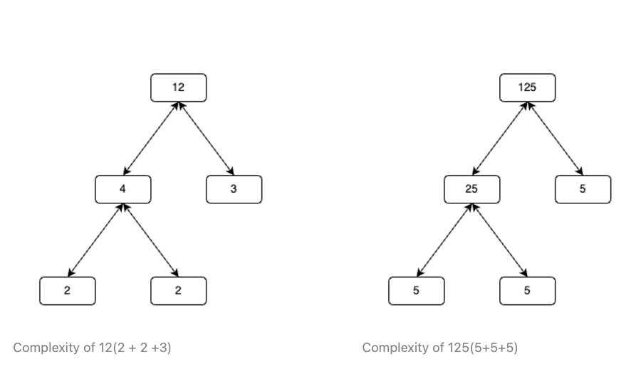
$$\begin{bmatrix}\omega^0 & \omega^0 & \omega^0 & \omega^0 \\\omega^0 & \omega^3 & \omega^6 & \omega^9 \\\omega^0 & \omega^6 & \omega^{12} & \omega^{18} \\\omega^0 & \omega^9 & \omega^{18} & \omega^{27} \\\end{bmatrix} \begin{bmatrix}A(0) \\A(3) \\A(6) \\A(9) \\\end{bmatrix} = \begin{bmatrix} A_1(0, 0) \\ A_1(1, 0) \\ A_1(2, 0) \\ A_1(3, 0) \\\end{bmatrix}$$

It’s clear that this is the exact same problem we started with, recall the matrix form of eq $(1)$. Hence the Cooley-Tukey FFT can be used to decompose this DFT further. Unfortunately in this example we end up with the same complexity since $2\cdot2 = 2+2$. But $N = 4$ is the only case where the sum of factors equals it’s product. In other cases recursive application of the Cooley-Tukey FFT provides significant efficiency gains when $N$ is highly composite:

$$\begin{split} N &= (r_0 \cdot r_1 \cdots r_{n-1}) \end{split}$$

Then the complexity of the algorithm becomes:

$$T = N(\sum_{i = 0}^{n-1} r_i)$$

The Cooley-Tukey FFT can also be combined with other FFT algorithms like the Good-Thomas FFT for factors that are coprime. This method completely eliminates the need for twiddle factors. Rader’s FFT can also be applied to DFT’s of prime lengths since they have no factors and can’t be decomposed further by the Cooley-Tukey algorithm.

Radix2FFT

What you popularly know as the Radix2FFT is actually another form of the Cooley-Tukey FFT. Since the Cooley-Tukey FFT can be applied recursively. Given the case when $N = 2^k$, you can continue to apply the the FFT until you reach a base case of two size-2 DFTs which can you evaluate and start to combine. This transformation yields the fastest time to compute the DFT:

$$\begin{split} T &= 2^k(2_0 + 2_1 + \dots + 2_k)\\ &= 2N\log_2 N \end{split}$$

Inverse FFT

The inverse FFT is the same as the FFT except it’s performed with inverse powers of the generator and finally multiplied by the inverse of the group order. This is given as:

$$A(k) = \frac{1}{N}\sum^{N-1}_{j=0}X(j) \cdot\omega^{-jk} \quad k = 0,1,\dots N-1.$$

(Proof is left as an exercise for the reader)

References

$^{[1]}$ An Algorithm for the Machine Calculation of Complex Fourier Series. James W. Cooley and John W. Tukey