Polynomial Commitments

Do not index

Special thanks to Alistair Stewart for the review and feedback on this article.

Polynomial commitment schemes are the foundational cryptographic primitive for things like computational integrity proofs (aka (ZK-)SNARKs) and verkle tries (a more efficient alternative to merkle-patricia tries). In this article i review their technical definition as well as their applications.

Polynomial commitments are a kind of commitment scheme that also allows for partial reveals, but with succint or logarithmic (wrt the prover complexity) proofs, irrespective of the size of the message. Polynomial commitment schemes are also a kind of vector-commitment scheme.

Vector commitment schemes enable a committer to commit to an ordered sequence of values in such a way that one can later open the commitment at specific positions (i.e., prove that is the -th committed message). For security, Vector Commitments are required to satisfy a notion referred to as positional binding which states that an adversary should not be able to open a commitment for two different values at the same position. Another property VCs must satisfy is succinctness, i.e. the size of the commitment string and of its openings has to be sublinear to the vector length. A merkle tree is a good example of a vector commitment.

A polynomial commitment scheme is a type of commitment scheme where rather than committing to an arbitrary sequence of bytes for a message we commit to a polynomial . Recall that a polynomial is of the form:

Where represents the coefficients of the polynomial.

Polynomial Interpolation

But why would we be committing to a polynomial in the first place!? The answer is, polynomial interpolation allows us to reverse engineer a polynomial function that encodes a message , by treating the elements contained within and it’s indices as a coordinate pair. i.e . Where is the index and is the value for the index in .

More formally, polynomial interpolation states that: given any arbitrary coordinate pairs , We can find or interpolate a polynomial of degree such that the evaluation of every over the polynomial produces . ie . There are a few ways to achieve polynomial interpolation, but two most popular methods are Lagrange Interpolation and Fast Fourier Transforms (FFT).

FFTs are a more efficient method for polynomial interpolation, especially when working with large sets of points. It involves transforming the set of points into a frequency domain representation, where the polynomial can be expressed as a series of sinusoidal functions.

Lagrange Interpolation on the other hand involves constructing a polynomial function that is a sum of smaller polynomial functions, each of which passes through a single point in the set. The Lagrange interpolation is formally represented by:

where is given as:

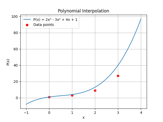
With this formula let’s perform the Lagrange interpolation of the data: . First we need to treat the data as a set of coordinates: .

We can graph the interpolated polynomial function to check if it does indeed pass through our data points.

At every point on the x-axis, corresponds with our data points on the y-axis

This example of course uses polynomials whose coefficients are members of the set of real numbers, In practice, polynomial interpolation & commitments are done over a finite field.

Back to polynomial commitment schemes, once we have a polynomial function that encodes a message , we can create a succinct commitment to the polynomial. Using this commitment, we can generate a proof for any given coordinate pair , such that a verifier who only has the commitment (and not the original polynomial ) can verify that in the original polynomial, the index does indeed correspond to value . Remember that this commitment is also succint, , i.e. the string representation of the polynomial commitment is less than the string representation of the original polynomial.

There are quite a few polynomial commitment protocols that exist today. These protocols have different tradeoffs that make them suitable for different applications. The most popular of them all is KZG.

KZG

I won’t be discussing the details of the advanced cryptographic primitives like finite fields, cyclic groups of prime orders or bilinear mappings and will be leaving them as an exercise for the reader.

The KZG commitment scheme, was introduced in 2010 by Aniket Kate, Gregory M. Zaverucha, and Ian Goldberg. Their paper outlines a protocol that produces constant-sized polynomial commitments and proofs of evaluation.

This protocol unfortunately requires a trusted set up, in that users must generate a secret parameter and discard this secret parameter otherwise malicious provers can create proofs of invalid evaluations. This trusted setup can be carried out in a distributed manner without relying on a central authority. All participants in the ceremony must collude to recover the secret parameter. However, if there is at least one honest participant who discards their share of the secret, the full secret cannot be reconstructed. This can be achieved using various MPC schemes that are available today.

The KZG commitment scheme at a high level works as follows:

Preliminaries

First we define as a finite field of prime order . Finite fields of prime order are simply a set given as where arithmetic operations over the elements of the set are performed modulo.

Next we define as a non-trivial bilinear mapping.

Finally, let be a generator for some pairing-friendly elliptic curve group where is a cyclic group of prime order :

Protocol

: Given some secret value , where . This method generates a proving key , that allows anyone commit to a polynomial of degree . This proving key, also called common reference string is of the form:

IMPORTANT: The secret value should not be recoverable, otherwise the prover can generate fraudulent proofs that can successfully fool the verifier.

: This outputs a constant-sized commitment to a polynomial for the public key .

More formally, Given some polynomial where , the commitment is of the form . Ideally, the prover doesn’t know , so instead they exploit a property of elliptic curve groups by using the proving key to compute which is equivalent to . It's also worth noting that this commitment is a single group element in and is why KZG commitments have constant sized commitments irrespective of the degree of .

: This outputs , where is a proof for the correct evaluation of at index . The prover computes the quotient polynomial given as:

Now given the quotient polynomial, the evaluation proof is given as . This proof is based on the polynomial remainder theorem and is also constant sized as it is also a single group element in .

: verifies that is indeed the evaluation at the index of the polynomial committed in . A verifier who has the commitment , the evaluation and a proof of evaluation can then compute:

If both pairings are equal, the verifier can be convinced that the prover does indeed know the full polynomial . It's also worth pointing out that the verifier always runs in constant time, regardless of the degree of the polynomial.

Applications

Polynomial commitments have many use cases, but in this section, we will only focus on applications that provide benefits to current blockchain architectures.

Verkle Tries

Armed with polynomial commitment schemes, we can revisit our merkle-patricia trie proof scheme and make them even more efficient. Recall that merkle patricia trie proofs require the hashes of all sibling nodes along the path to the value. This means that proof sizes are where is the arity of the nodes.

We can remove the need for these sibling nodes in our proofs by instead performing a polynomial interpolation over the branch nodes and producing a polynomial commitment rather than a cryptographic hash. Then with this constant-sized commitment, we can produce constant-sized membership proofs for any of the child nodes in the branch node. This scheme is popularly known as the Verkle (vector commitment merkle) trie .

Since polynomial commitments produce constant-sized membership proofs irrespective of the set size, this allows us to shorten the height of the verkle tree and achieve a smaller set of polynomial evaluation proofs. To accomplish this, we increase the arity of each branch node from 16 (as in Merkle Patricia Tries) to up to 2048. This effectively reduces the number of polynomial evaluation proofs needed to prove membership for any item in the tree. We can even further reduce the proof size for a Verkle tree by using KZG multiproofs. This allows us to reduce a set of KZG proofs to a single group element .

Verkle trees enable higher bandwidth cross-chain messaging by producing state proofs for cross-chain messages of a constant size. They also have noteworthy applications in parachain scalability. As discussed in a previous article, parachain blocks are re-executed by the relay chain to achieve validity guarantees. However, by leveraging verkle trees, we can create more room for parachain transactions in the proof of validity payload that gets sent to the relay chain.

Proofs of computational integrity

Polynomial commitments can also be used to obtain cryptographic proofs of computational integrity. This allows a prover to convince a verifier that they have correctly executed a mutually known program with some (possibly private) inputs, and that this program has yielded some given outputs.

Proofs of computational integrity are powered by a combination of polynomial IOPs and polynomial commitment schemes. Functionally, a polynomial IOP allows a prover to convince a verifier that they know some computation trace for which a set of polynomial constraints holds. These polynomial constraints are known by the verifier ahead of time through a commitment to all constraint polynomials in the program. This computation trace can then be generated by a process known as arithmetization.

I won’t be discussing in-depth how the Polynomial IOPs work and will leave it as an exercise to the reader.

Through arithmetization, a prover can generate a two-dimensional array that encodes how different variables in a program change over time. This process uses a register-based model in which variables are stored in registers. The prover then turns on and off different gates for variables in the registers using polynomial constraints that evaluate to zero. The verifier, who has a commitment to all of the polynomial constraints, will query at any random point to confirm that the constraint polynomial evaluates to zero. If this check is satisfied, the verifier can conclude with a high probability that the prover does indeed possess a valid computation trace for the given inputs. (This zero-check is based on the Schwartz-Zippel lemma).

This is a powerful primitive that immensely scales blockchains. By running multiple state machines concurrently and producing "validity proofs" that confirm the correct execution of their state transition function, a consensus layer can verify these proofs cheaply and trust that they accurately describe a valid state transition without needing to re-execute the full block.

Proofs of computational integrity can also be applied to consensus-verifying bridges. They provide a cost-effective and indirect way to verify consensus proofs for a counter-party blockchain, which usually requires signatures from a supermajority of all validators. Naively verifying this consensus proof on-chain can be too expensive due to the lack of necessary host functions/precompiles or because of the sheer size of the super-majority set. Pairing polynomial commitments with polynomial IOPs for consensus verification can produce constant-sized proofs, regardless of the size of the consensus proof. This compression allows for a potentially massive set of signatures to be condensed into a constant-sized proof that can be verified in constant time.

Summary

We have reviewed polynomial commitments, how they work, and how they underpin advancements in blockchain scalability through efficient state proof schemes, consensus-verifying bridges that are cheap to maintain and verifiable state machines which can scale blockchain throughput to thousands of transactions per second.

References

A. Kate, G. M. Zaverucha, I. Goldberg, Polynomial Commitments

Seun Lanlege, State (Machine) Proofs

Verkle Trees, John Kuszmaul

Dankrad Feist, Kate Polynomial Commitments